Exercises
1 The basics
1.1 Install and set up R and RStudio
Install R
First, install R at this link: https://cran.r-project.org/mirrors.html. Choose a mirror approximately close to you geographically, and then choose the option corresponding to your operating system:
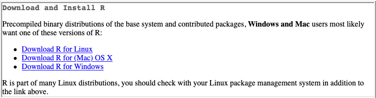
Follow all the operating system-specific instructions.
Congratulations! 🥳 You have R installed! That means you could write an R script and run it. But let’s make things a lot easier by downloading RStudio, which will keep us organized and supply us with lots of shortcuts.
Install R Studio
You can download RStudio at this link: https://rstudio.com/products/rstudio/download/. Choose the RStudio Desktop free version on the left:
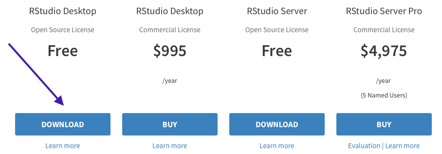
And then the blue download button near the top should match your operating system. If not, you can choose from the list below it.
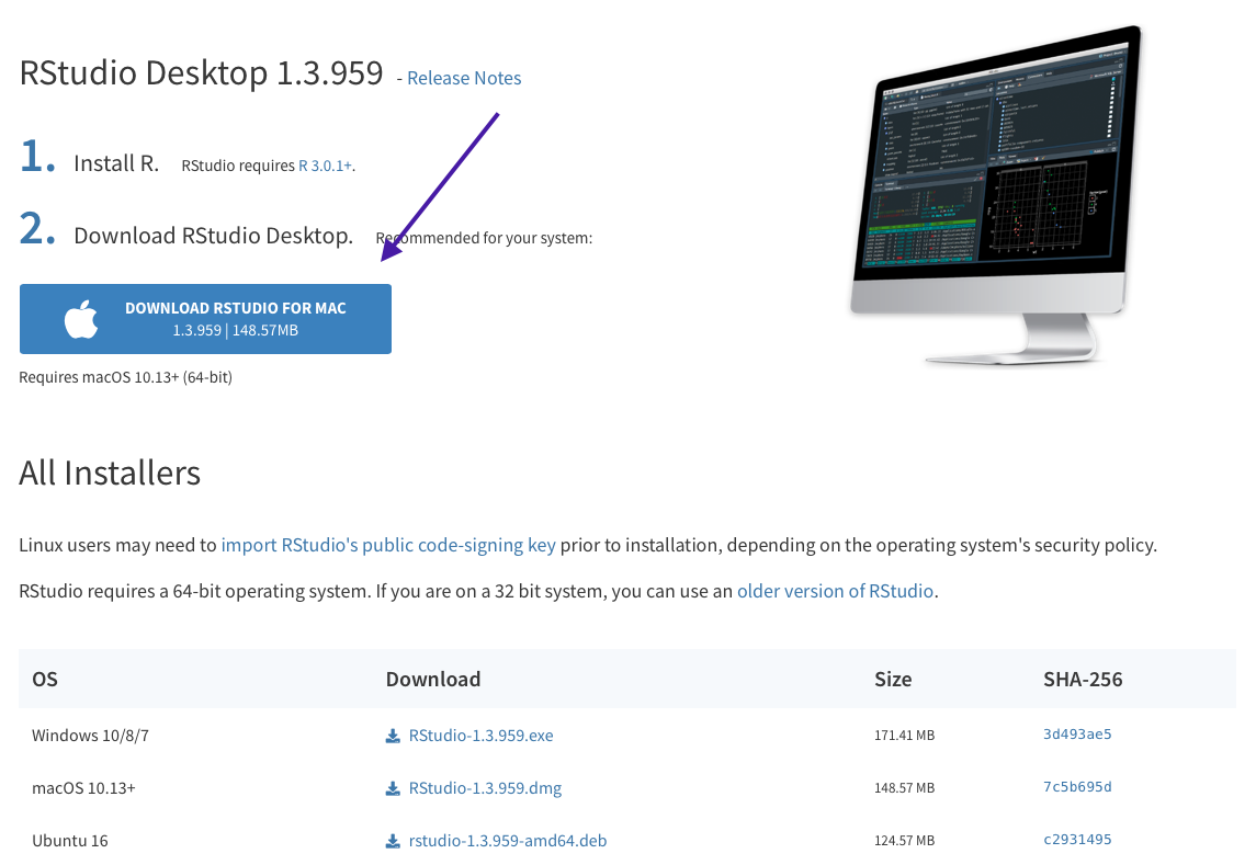
Again follow the instructions for download. Now open up RStudio. It should automatically be connected with R!
Personalize R Studio
There’s a lot you can do to personalize RStudio. Feel free to explore all the options and do what you want with it.1 You can do a lot of personalization through the “Global Options” menu under “Tools”. Here’s what it looks like on Windows:
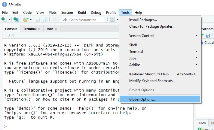
🛑 One change that I will request that you make is to change what RStudio does when you restart R. You want your settings to look like this:
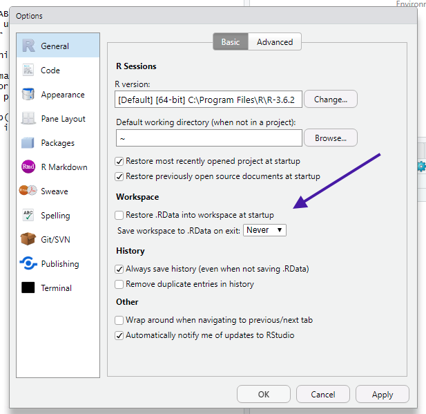
(You will have to restart RStudio.)
The reason I want you to set things up this way is because it’s really easy to make mistakes if you let R remember the data and packages you had loaded the last time you used it.
1.2 Install and load packages
Install the tidyverse package
Open up RStudio. In the console, type in install.packages("tidyverse") and press enter. Then wait a while. Voilà! You have just installed a lot of super useful packages.
You ran that code in the console because it’s not something you’ll need to run again or look back at. When you are loading a package, you’ll want to do that from a script. You’ll want a record of the fact that you loaded the package so that if you or someone else wants to rerun the code, they’ll have the appropriate packages.
If you’re trying to run code that requires a package you haven’t installed, either RStudio will suggest they do so (because RStudio is magical 🧙), or you’ll get an error when you run library(package_name). In fact, here’s what happens when you try to load that package (which I haven’t installed because it doesn’t exist!)
library(package_name)Load the tidyverse package
To open a new R script, choose “File” -> “New File” -> “R Script”, or simply click on the button with a green plus sign at the upper-left corner of the window. This is a blank document that you can write code in and save to come back to.
In that document, write:
# load packages
library(tidyverse)
The first line is a comment, which won’t run when you run the script. Comments in R start with # and can include whatever they want after that. To comment out multiple lines, simply preface each one with #. (Highlighting them all and using Cmd/Ctrl + Shift + c is faster!)
If you highlight both lines, or just put your cursor on the end of the second, and then press Cmd/Ctrl + Enter, the code will run. You should see some text show up in the console.
# load packages
library(tidyverse)The first section is telling you which packages are actually being loaded with the “mega-package” tidyverse, and the second section is telling you that there are some functions loaded, specifically from the dplyr package, that have the same names as those in the stats package. The stats package is on that automatically is loaded with R, so you’ll always have these conflicts.
In this class, we’ll be using the dplyr versions of those functions, so this isn’t a problem. In general, if you want to be specific about which package a function comes from, you can write, e.g., stats::filter(x), so that R knows to use the version of the filter() function from the stats package.2
Refresh R and load another package
Now let’s see what happens when we restart R. There are two ways to do this:
- Literally quit RStudio, and open it back up again.
- Go to
Session -> Restart Rin the menu bar. There’s also a keyboard shortcut you can memorize.3
Now, open a new file, and type in and run this code:
ggplot(mpg, aes(displ, hwy, colour = class)) +
  geom_point() +
  geom_smooth(se = FALSE, method = lm)
You should get this error:
If you didn’t, you didn’t correctly restart R! 🤦 Try again.
Now add the necessary library() call and run the whole thing again:
library(ggplot2)
ggplot(mpg, aes(displ, hwy, colour = class)) +
  geom_point() +
  geom_smooth(se = FALSE, method = lm, formula = "y ~ x")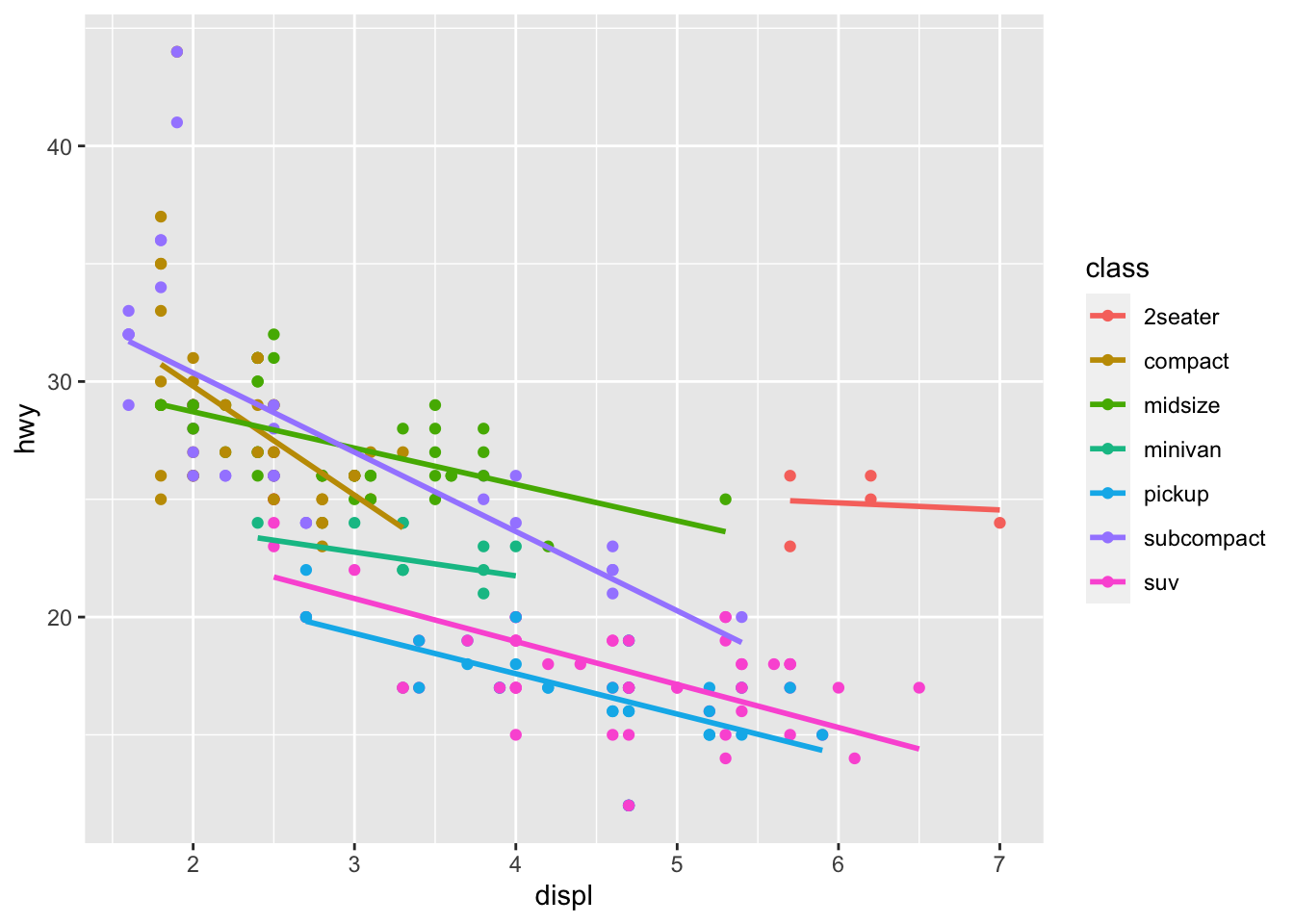
You should see this figure pop up in the Plots window!
You can quit RStudio and you don’t have to save this file. We’ll be back to figures like that next week! 📊
1.3 Organize your files
Click here to download this week’s files. You’ll have to unzip it to access the files inside. This is a little annoying if you are on Windows, but you can follow these instructions:
Unzip a folder in Windows
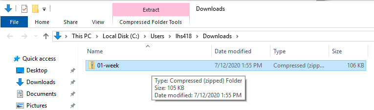
- Save the zip file to Downloads. You should see something like this:
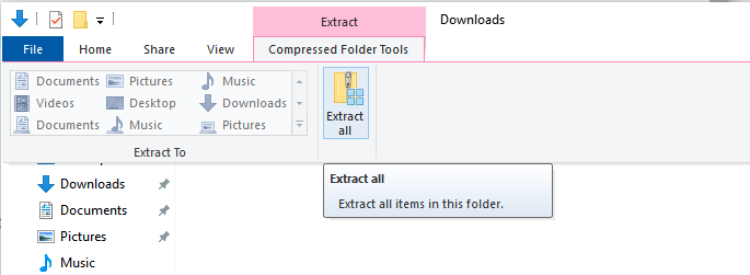
- Go up to
Extract -> Compressed Folder Tools -> Extract All, like this:
- Just leave the default folder for extraction. We’ll move it later.
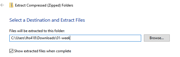
- Now you’ll see that you’re in the
Downloads/01-week/folder, in which there’s another folder called01-week. We want this one. You can ignore the_MACOSXone (that’s just there because I made it on a Mac). Move this01-weekfolder to wherever you’re keeping files for this class, e.g., in a folder calledR-courseas in the slides. (Here I’m moving it to a folder calledR– don’t do this, name it something better!)
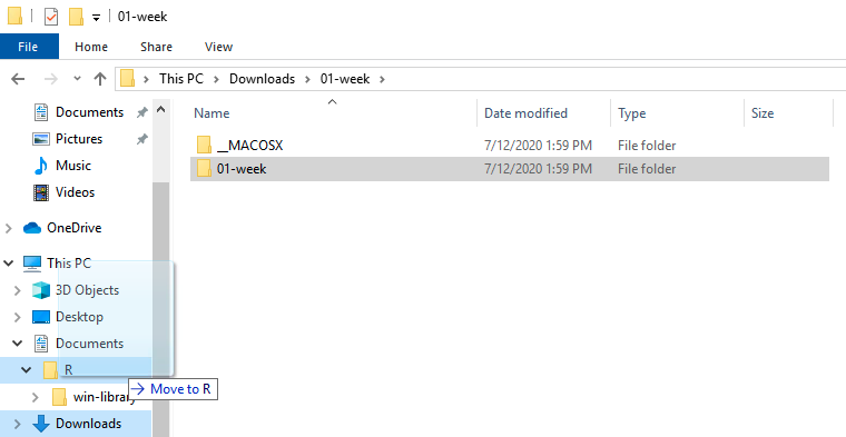
- Then, back in your downloads folder, you can delete both folders called
01-week, because you’ve moved out the stuff you need.
Unzip a folder on a Mac
- Go to
Downloads, or wherever you have files set to download. You’ll see something like this:
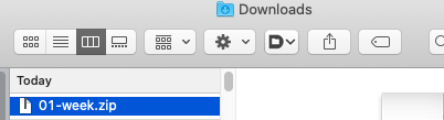
- Double click to unzip. You’ll now have the unzipped folder as well. Move that one to wherever you’re keeping files for this class, e.g., in a folder called
R-courseas in the slides. You can delete01-week.zip!
Open up an R project
Inside the 01-week folder, you’ll see a file called 01-week.Rproj. If you’re on Windows, it should look like this:

Double-clicking on it should open up RStudio. If not, follow these instructions:
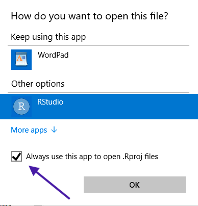
Open up an R project in Windows
Right-click on the file, then choose Open with -> Choose another app. Make sure to Choose another app even if RStudio shows up in the Open with menu, because you want to change the settings for all .Rproj files. Find RStudio and change the settings like this:
Open up an R project on a Mac
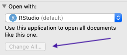
Don’t do right-click -> Open with because you want to change the settings for all files. Instead, right-click -> Get info (right-click for you may be a two-fingered click on a trackpad, or cmd/ctrl + click). Go down to Open with, find RStudio, and then make sure to check Change all so you don’t have to do this again:
Folder structure
Check out your files in the Files viewpane (one of the tabs by Plots). You should see all the materials for this week! They include:
01-week.Rproj: We’ve covered what this does01-exercise.html: This is essentially what you see on this webpage, but you can open it up in your browser if you don’t have an internet connection01-exercise.Rmd: This is the R Markdown file I wrote to generate the webpage, if you want to see the code behind it. You can open it up and clickKnitat the top of the RStudio window if you want to generate it yourself (you might need to install some packages). Learn more about R Markdown here.01-todo.R: This is the R script you’ll be working with in the next session!
Also check to make sure that you’re in the correct working directory. You can find that at the top of your console pane. It should look something like this:4

If not, you didn’t open RStudio via the 01-week.Rproj file. 🤦 Close RStudio and try again!
1.4 Run some R code!
Work through the code in 01-todo.R. You should run the code line-by-line, from a fresh R session (restart if you need to), paying attention to what happens in each of your RStudio windows as you do.
Then answer these questions (also included at the end of the script):
- Extract
645fromvalsusing square brackets. - Extract
"rhino"fromcharsusing square brackets. - You saw how to extract the second row of
mat. Figure out how to extract the second column. - Extract
183frommatusing square brackets. - Figure out how to get the following errors:
incorrect number of dimensionssubscript out of bounds
Save your 01-todo.R script so you can come back to it later! We’ll go over any questions you have during lab. See you then! 👋
For example, I use the Fira Code font. Instructions to install can be found here. Beyond the themes that come pre-installed with RStudio, there are a variety of others available with the
rsthemespackage here. You can also make your own theme! There’s more information in this article.↩︎See also the
conflictedpackage if this turns out to be a problem often.↩︎You can see all the other keyboard shortcuts, or change them, by going to
Tools -> Keyboard Shortcuts HelporModify Keyboard Shortcuts.↩︎My “c” key wasn’t working when I named the “R-course” folder!↩︎