6.1 File paths

We talked this week about making file paths work in R. This is especially important if you’re sharing your code with everyone. If you set your working directory via setwd() or hard-code another path into your code, it’s definitely not going to work on my computer.

A famous blog post about this (well, as famous as blog posts about R can be) can be read here.

How did you make these file paths work?

library(tidyverse)
library(knitr)
nlsy <- read_csv("nlsy.csv")

# this function adds a static image
include_graphics("figure1.jpg")

read_rds("table1.rds") %>%
  kable() # this function prints nicer tables in R Markdown

By the way, you can change the directory in which an R Markdown document is knitted using the arrow by the Knit button. You can also use the settings to change the default. But if you use the here package it won’t matter what you do!

One thing that is helpful to know when you’re working interactively, is how to navigate around file paths. If you need to go up a level, you use two dots to do so. So in the code below, we go down two levels from the top-level directory, then have to go up two levels and down two different levels to access the data. See why project directories and the here package make everything easier?!

proj_wd <- getwd()
setwd("figures/super important")
nlsy <- read_csv("../../data/raw/nlsy.csv")
# ahhh take us back to where we started from!
setwd(proj_wd)

6.2 Missing data

The nlsy.csv file includes all 12,687 participants of the NLSY-79. Read in the data once without specifying the values that indicate missingness. Explore the data and find them all. Then read in the data again, using the na = argument in read_csv() to read them in as NA’s.

# skip = 1 means to skip the first row, which were the original col names
nlsy <- read_csv(here::here("data", "raw", "nlsy.csv"), skip = 1, col_names = c(
  "glasses", "eyesight", "sleep_wkdy", "sleep_wknd",
  "id", "nsibs", "samp", "race_eth", "sex", "region",
  "income", "res_1980", "res_2002", "age_bir"
))

How can we explore the data to get an idea of what values mean that variable is missing?

summary(nlsy)

#>      glasses          eyesight          sleep_wkdy       sleep_wknd    
#>   Min.   :-4.000   Min.   :-4.00000   Min.   :-4.000   Min.   :-4.000  
#>   1st Qu.:-4.000   1st Qu.:-4.00000   1st Qu.:-4.000   1st Qu.:-4.000  
#>   Median : 0.000   Median : 1.00000   Median : 6.000   Median : 6.000  
#>   Mean   :-1.026   Mean   : 0.04004   Mean   : 2.523   Mean   : 2.886  
#>   3rd Qu.: 1.000   3rd Qu.: 2.00000   3rd Qu.: 7.000   3rd Qu.: 8.000  
#>   Max.   : 1.000   Max.   : 5.00000   Max.   :19.000   Max.   :24.000  
#>         id            nsibs             samp           race_eth    
#>   Min.   :    1   Min.   :-3.000   Min.   : 1.000   Min.   :1.000  
#>   1st Qu.: 3172   1st Qu.: 2.000   1st Qu.: 5.000   1st Qu.:2.000  
#>   Median : 6344   Median : 3.000   Median : 9.000   Median :3.000  
#>   Mean   : 6344   Mean   : 3.844   Mean   : 8.174   Mean   :2.434  
#>   3rd Qu.: 9515   3rd Qu.: 5.000   3rd Qu.:12.000   3rd Qu.:3.000  
#>   Max.   :12686   Max.   :29.000   Max.   :20.000   Max.   :3.000  
#>        sex            region           income         res_1980      
#>   Min.   :1.000   Min.   :-4.000   Min.   :   -3   Min.   :-5.0000  
#>   1st Qu.:1.000   1st Qu.: 2.000   1st Qu.: 2853   1st Qu.:-4.0000  
#>   Median :1.000   Median : 3.000   Median : 7955   Median :-4.0000  
#>   Mean   :1.495   Mean   : 2.424   Mean   :11819   Mean   : 0.5317  
#>   3rd Qu.:2.000   3rd Qu.: 3.000   3rd Qu.:18000   3rd Qu.:11.0000  
#>   Max.   :2.000   Max.   : 4.000   Max.   :75001   Max.   :16.0000  
#>      res_2002         age_bir       
#>   Min.   :-5.000   Min.   :-998.00  
#>   1st Qu.:-5.000   1st Qu.:  -5.00  
#>   Median :11.000   Median :  -5.00  
#>   Mean   : 4.914   Mean   : -96.36  
#>   3rd Qu.:11.000   3rd Qu.:  23.00  
#>   Max.   :19.000   Max.   :  52.00

ggplot(nlsy) +
  geom_histogram(aes(age_bir))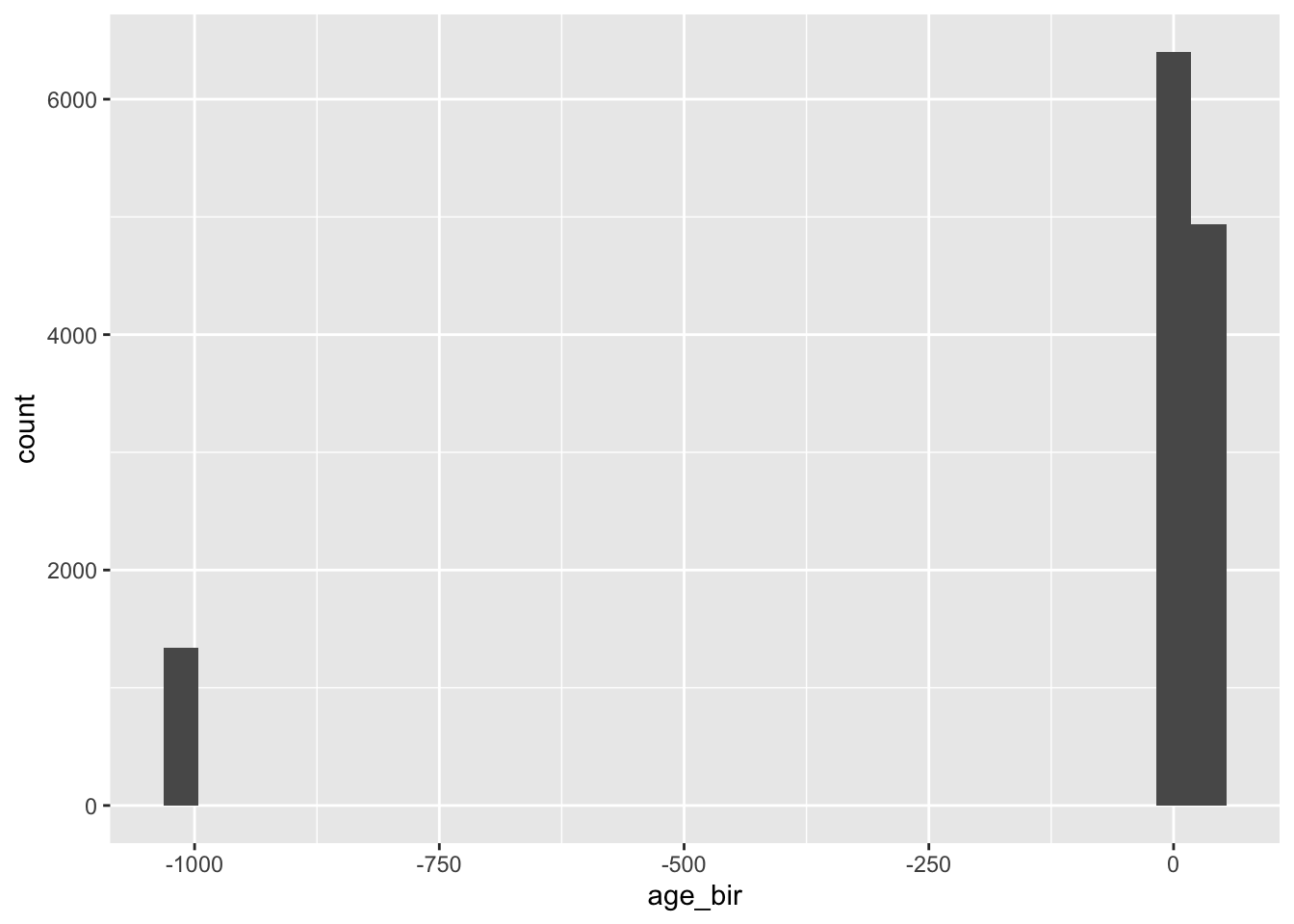

count(nlsy, nsibs)

#>  # A tibble: 25 x 2
#>     nsibs     n
#>     <dbl> <int>
#>   1    -3    14
#>   2    -2     3
#>   3    -1     1
#>   4     0   362
#>   5     1  1611
#>   6     2  2530
#>   7     3  2412
#>   8     4  1783
#>   9     5  1198
#>  10     6   933
#>  # … with 15 more rows

Reread the data with the missing values specified:

nlsy <- read_csv(here::here("data", "raw", "nlsy.csv"), skip = 1, 
                 na = c("-998", "-5", "-4", "-3", "-2", "-1"),
                 col_names = c(
  "glasses", "eyesight", "sleep_wkdy", "sleep_wknd",
  "id", "nsibs", "samp", "race_eth", "sex", "region",
  "income", "res_1980", "res_2002", "age_bir"
))

Check again to see if anything’s off:

summary(nlsy)

#>      glasses         eyesight       sleep_wkdy       sleep_wknd    
#>   Min.   :0.000   Min.   :1.000   Min.   : 0.000   Min.   : 0.000  
#>   1st Qu.:0.000   1st Qu.:1.000   1st Qu.: 6.000   1st Qu.: 6.000  
#>   Median :0.000   Median :2.000   Median : 7.000   Median : 7.000  
#>   Mean   :0.461   Mean   :2.064   Mean   : 6.567   Mean   : 7.163  
#>   3rd Qu.:1.000   3rd Qu.:3.000   3rd Qu.: 8.000   3rd Qu.: 8.000  
#>   Max.   :1.000   Max.   :5.000   Max.   :19.000   Max.   :24.000  
#>   NA's   :4236    NA's   :4242    NA's   :4860     NA's   :4867    
#>         id            nsibs             samp           race_eth    
#>   Min.   :    1   Min.   : 0.000   Min.   : 1.000   Min.   :1.000  
#>   1st Qu.: 3172   1st Qu.: 2.000   1st Qu.: 5.000   1st Qu.:2.000  
#>   Median : 6344   Median : 3.000   Median : 9.000   Median :3.000  
#>   Mean   : 6344   Mean   : 3.854   Mean   : 8.174   Mean   :2.434  
#>   3rd Qu.: 9515   3rd Qu.: 5.000   3rd Qu.:12.000   3rd Qu.:3.000  
#>   Max.   :12686   Max.   :29.000   Max.   :20.000   Max.   :3.000  
#>                   NA's   :18                                       
#>        sex            region          income         res_1980     
#>   Min.   :1.000   Min.   :1.000   Min.   :    0   Min.   : 1.000  
#>   1st Qu.:1.000   1st Qu.:2.000   1st Qu.: 5900   1st Qu.: 6.000  
#>   Median :1.000   Median :3.000   Median :10700   Median :11.000  
#>   Mean   :1.495   Mean   :2.547   Mean   :14707   Mean   : 8.896  
#>   3rd Qu.:2.000   3rd Qu.:3.000   3rd Qu.:20000   3rd Qu.:11.000  
#>   Max.   :2.000   Max.   :4.000   Max.   :75001   Max.   :16.000  
#>                   NA's   :239     NA's   :2491    NA's   :8186    
#>      res_2002        age_bir     
#>   Min.   : 1.00   Min.   :10.00  
#>   1st Qu.:11.00   1st Qu.:20.00  
#>   Median :11.00   Median :23.00  
#>   Mean   :11.28   Mean   :24.38  
#>   3rd Qu.:11.00   3rd Qu.:28.00  
#>   Max.   :19.00   Max.   :52.00  
#>   NA's   :4962    NA's   :6743

ggplot(nlsy) +
  geom_histogram(aes(age_bir))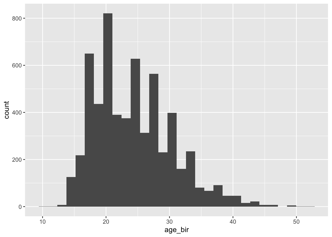

count(nlsy, nsibs)

#>  # A tibble: 23 x 2
#>     nsibs     n
#>     <dbl> <int>
#>   1     0   362
#>   2     1  1611
#>   3     2  2530
#>   4     3  2412
#>   5     4  1783
#>   6     5  1198
#>   7     6   933
#>   8     7   634
#>   9     8   421
#>  10     9   289
#>  # … with 13 more rows

There are certainly some outliers we might want to investigate, but nothing else coded as missing.

(Obviously, these missing values are noted in the data dictionary. You shouldn’t have to guess what the missing values are when you’re working with real data – ask someone who knows, instead!)

Now imagine you’re interested in how the number of siblings relates to one’s age when they have their first child. Create a dataset to study this question:

• Assume that if the number of siblings is missing, they have 0
• Create a variable that is 1 if someone has kids, and 0 otherwise
• Create a dataset containing id, the sibling/child variables of interest, and income.
• Subset the data to exclude people who are missing income.

for_analysis <- nlsy %>%
  mutate(
    nsibs = case_when( # or ifelse(is.na(nsibs), 0, nsibs)
      is.na(nsibs) ~ 0,
      TRUE ~ nsibs
    ),
    has_kids = case_when( # or ifelse(!is.na(age_bir), 1, 0)
      !is.na(age_bir) ~ 1,
      TRUE ~ 0
    )
  ) %>%
  select(id, nsibs, has_kids, age_bir, income) %>%
  filter(!is.na(income))

6.3 Questions?!?!