Exercises
2 Figures
Prepare
Download the materials for this week’s exercises here. Once you’ve unzipped (and extracted, if you’re on Windows) the file and moved the folder wherever you want, open up a new RStudio session using the 02-week.Rproj file. You should have nothing in your environment. If you’re having trouble with this, look back at last week’s exercises for guidance.
Then you’ll need to load the tidyverse package and read in the data. In lab we read it in from a url, this time I gave you the data in the zipped folder. The function to read it in is the same:
library(tidyverse)
nlsy <- read_csv("nlsy_cc.csv")
2.1 Intro to ggplot2
Make a scatterplot
Make a scatter plot of the relationship between hours of sleep on weekends and weekdays. Color it according to region (where 1 = northeast, 2 = north central, 3 = south, and 4 = west). Use the code from the example below to get started!
ggplot(data = nlsy) +
  geom_point(aes(x = income, y = age_bir, color = factor(eyesight))) +
  scale_color_brewer(palette = "Set1", name = "Eyesight",
                     labels = c("Excellent", "Very Good", "Good",
                                "Fair", "Poor"))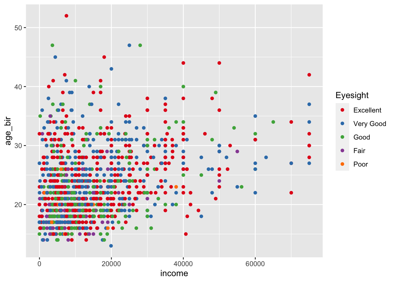
Jittering
Using your plot from the previous question, replace geom_point() with geom_jitter(). What does this do? Why might this be a good choice for this graph? Play with the width = and height = options within geom_jitter(). This site may help: https://ggplot2.tidyverse.org/reference/geom_jitter.html
Shapes
Use the shape = argument to map the sex variable to different shapes. Change the shapes to squares and diamonds. (Hint: how did we manually change colors to certain values? This page might also help:
https://ggplot2.tidyverse.org/articles/ggplot2-specs.html)
Explore!
Using a structure like this, you can explore changing what’s in the <>.
- Use either the resources in the slides (now also on the resources page), or just start typing e.g.,
geom_orscale_colorand choose one of the autocompletes. - Depending on what you choose, different arguments might be required/allowed. For example,
geom_point()requires bothx =andy =, butgeom_histogram()onlyx =. You can usehelp(geom_point)for guidance, under the “Aesthetics” section. - What happens if you include
color =both within and outside of theaes()argument? What happens if you use an actual color, like"blue"inside? Or a variable name outside? - It might be helpful for you to keep a script with all the different things you try, with a comment about whether or not it worked and what you did.
ggplot(data = nlsy) +
  geom_<>(aes(x = <>, y = <>, color = <>, ...), color = <>, ...) +
  scale_color_<>(name = <>, ...)
2.2 Facets
First we made a graph faceted by columns. Then we switched to rows. Try that out with this code. Try out another variable to facet by, instead of region. What if we facet by both columns and rows? You can also play around with the margins = and the scales = arguments. Use help(facet_grid) to find out more.
ggplot(data = nlsy) +
  geom_bar(aes(x = nsibs)) +
  labs(x = "Number of siblings") +
  facet_grid(cols = vars(region), margins = TRUE, scales = "free_y")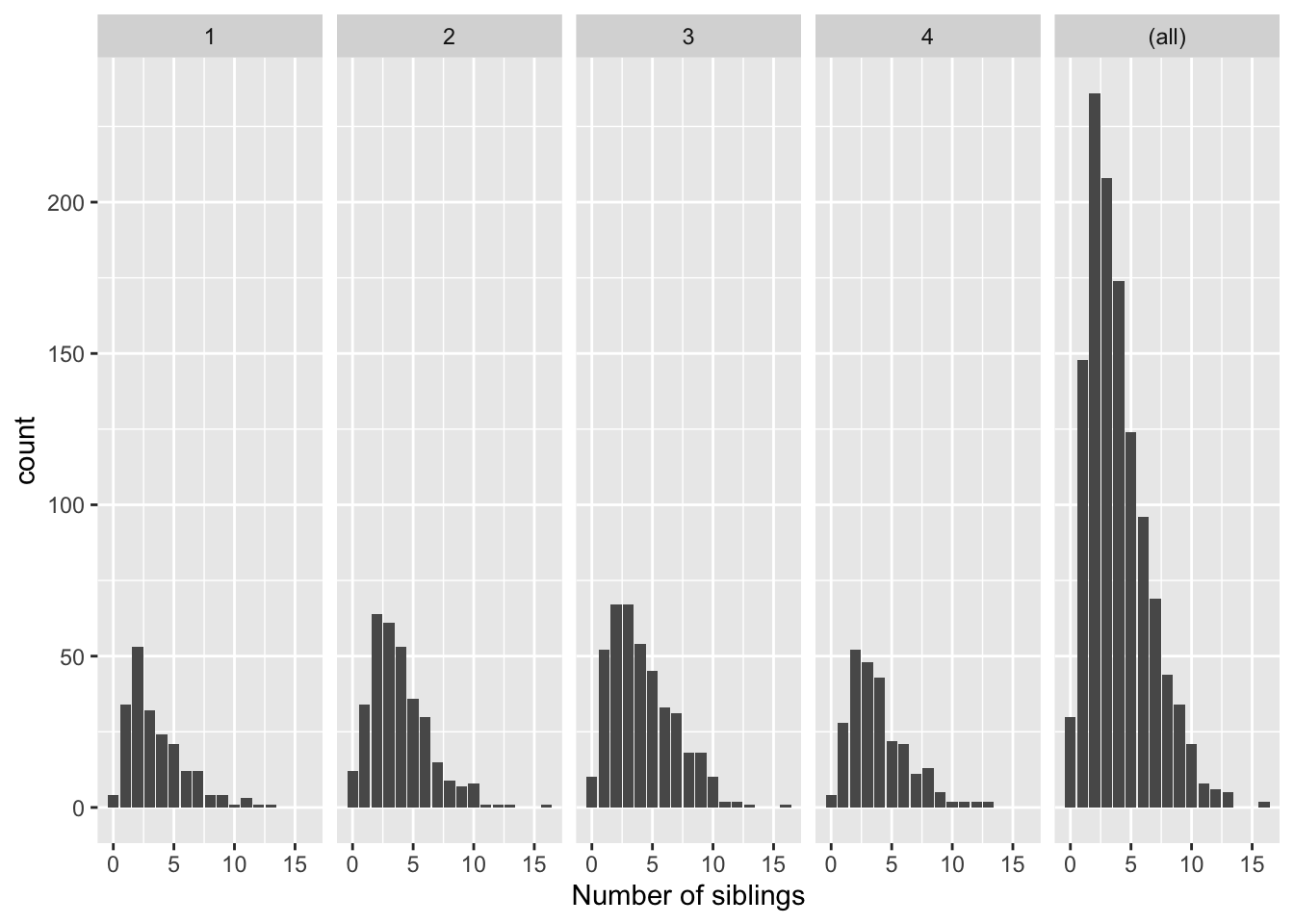
We also saw that we could (maybe) make better use of space with facet_wrap(). Try changing the variable we’re facetting by (region), and the ncol = argument. Alternatively, you can specify the number of rows with nrow =.
ggplot(data = nlsy) +
  geom_bar(aes(x = nsibs)) +
  labs(x = "Number of siblings") +
  facet_wrap(vars(region),
             ncol = 3)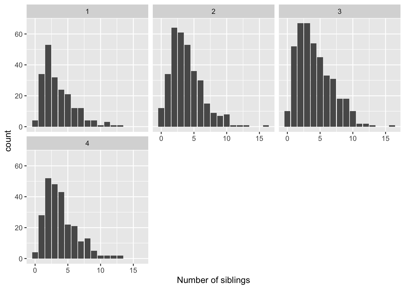
We also learned to make a histogram, with a bin for every $1,000 of income. Try out some different binwidth = or bins = argument. Or leave it out and see the warning you get!
ggplot(data = nlsy) +
  geom_histogram(aes(x = income), binwidth = 1000)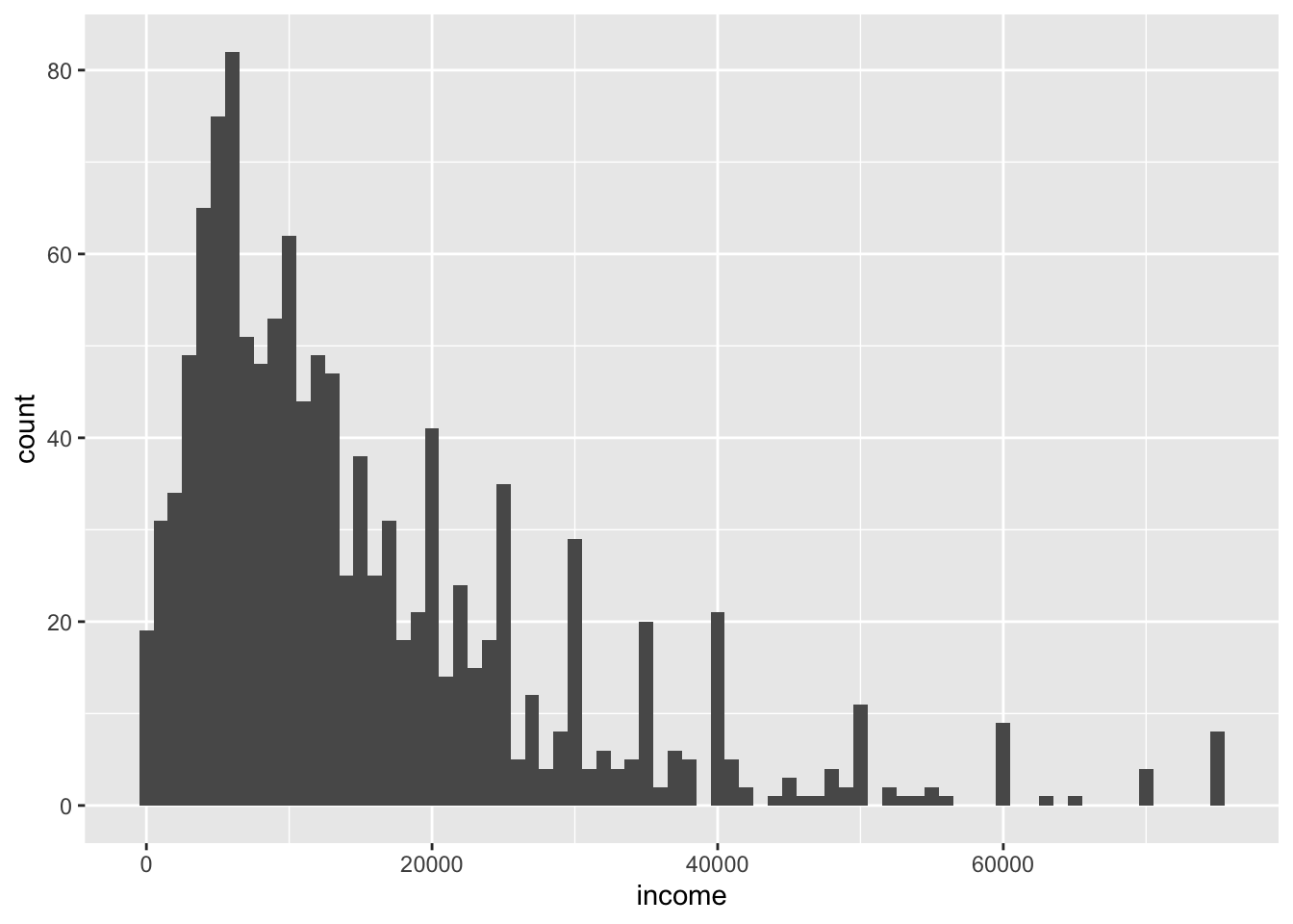
Density histograms
When we’re comparing distributions with very different numbers of
observations, instead of scaling the y-axis like we did with the
facet_grid() function, we might want to make density histograms, where instead of the count of observations along the y-axis, we have the density (i.e., the histogram is scaled so that its entire area adds up to 1). Use google to figure out how to make a density histogram of income. Facet it by region.
Color your histograms
Make each of the regions in your previous histogram a different color. (Hint: compare what col = and fill = do to histograms).
scale_x_...
Instead of a log-transformed x-axis, make a square-root transformed x-axis. See what other options for the x-axis you have, using the autocomplete in RStudio.
Label your x-axis
Doing the last part squishes the labels on the x-axis. Using the breaks = argument that all the scale_x_...() functions have, make labels at 1000, 10000, 25000, and 50000.
2.3 Saving your work
Here’s a plot to start you off. Look through each line and make sure you understand what it’s doing.
ggplot(data = nlsy) +
  geom_boxplot(aes(x = factor(sleep_wknd), y = sleep_wkdy,
                   fill = factor(sleep_wknd))) +
  scale_fill_discrete(guide = FALSE) +
  labs(x = "hours slept on weekends",
       y = "hours slept on weekends",
       title = "The more people sleep on weekends,
       the more they sleep on weekdays",
       subtitle = "According to NLSY data") +
  theme_classic()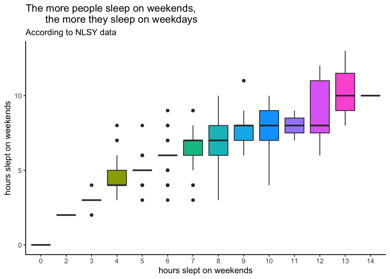
Using ggsave()
Using the plot above as guidance, change at least 3 elements, if not more! Then save it using the code below. These are probably not the right dimensions for your plot, so experiment! You can also change from pdf to e.g., png by changing the file name. Look in the files pane to see where your saved plot shows up.
ggplot()

ggsave(filename = "my_plot.pdf", height = 8, width = 4)
Storing your plot as an object
That function will automatically save the last plot you made. If you’re making lots of plots, you should store them and refer to them by name. Try that with a new plot here. Notice what happens in the plots pane, and in the environment pane, when you do so.
new_plot <- ggplot()

ggsave(plot = new_plot, filename = "another_plot.png")
Challenge: Recreate the plot from the slides
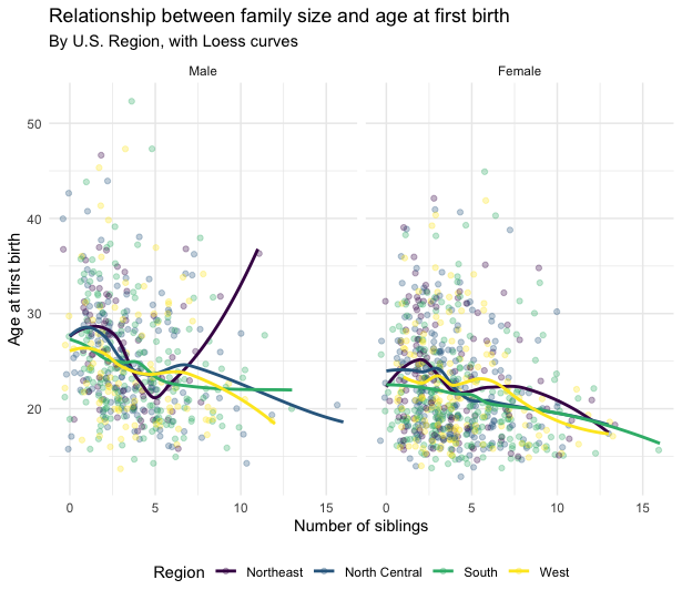
This will definitely require some Googling (reminder: I have to Google something for almost every plot I make!) so is a challenge! See how close you can get. We’ll also be working on this in lab, so don’t worry if you don’t get very far!